Get transmembrane tendency#

Evaluating amino acid insertion and propensity scores for lipid membranes.

The function molsysmt.physchem.get_transmembrane_tendency() returns empirical free-energy insertion propensities for residues in lipid bilayers using two published scales:

'zhao': Free-energy-based insertion scale from Zhao & London (2006).
'senes': Statistical pseudo-potential scale from Senes et al. (2007).

Added in version 1.0.0.

API documentation

Follow this link for a detailed description of the input arguments, raised errors, and returned objects of this function: molsysmt.physchem.get_transmembrane_tendency().

Basic usage#

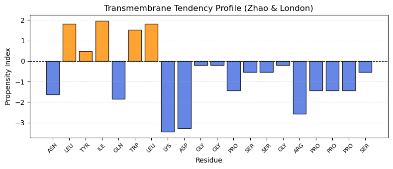
By default (definition='zhao'), free-energy-based insertion tendencies into lipid bilayers are reported (positive values indicate membrane preference, negative values indicate aqueous preference):

import molsysmt as msm
import matplotlib.pyplot as plt

molsys = msm.convert(msm.systems['Trp-Cage']['1l2y.h5msm'])

Note

Demo Systems Catalog

This tutorial uses demonstration datasets provided by MolSysMT. To explore the full catalog of bundled systems, forms, and file paths, visit the Demo Systems guide.

We query the Zhao & London transmembrane propensity scores and plot the sequence profile:

tt = msm.physchem.get_transmembrane_tendency(molsys, element='group', definition='zhao')
group_names = msm.get(molsys, element='group', name=True)

fig, ax = plt.subplots(figsize=(8, 3.5))
colors = ['darkorange' if val > 0 else 'royalblue' for val in tt]
ax.bar(range(len(tt)), tt, color=colors, edgecolor='black', alpha=0.8)
ax.axhline(0, color='black', linestyle='--', linewidth=0.8)
ax.set_xticks(range(len(tt)))
ax.set_xticklabels(group_names, rotation=45, fontsize=8)
ax.set_title('Transmembrane Tendency Profile (Zhao & London)')
ax.set_xlabel('Residue')
ax.set_ylabel('Propensity Index')
ax.grid(True, linestyle='--', alpha=0.4, axis='y')
plt.tight_layout()
plt.show()

../../../../_images/1f52870469a8823faa4abd76bbf06ad3bf05e0686de6a7f26e5de4f61359a5d6.png

Alternative transmembrane scales#

Setting definition='senes' extracts statistical pseudo-potential propensities derived from transmembrane helix structures:

tt_senes = msm.physchem.get_transmembrane_tendency(molsys, element='group', definition='senes')
print('Senes propensity scores:\n', tt_senes)

Senes propensity scores:
 [[0.89, 12.78, 6.28], [-0.64, 17.34, 8.61], [-0.42, 13.04, 6.2], [-0.56, 14.34, 10.69], [1.21, 10.46, 2.59], [-0.85, 11.65, 7.2], [-0.64, 17.34, 8.61], [1.66, 11.11, 2.09], [1.19, 14.25, 8.98], [-0.01, 13.86, 6], [-0.01, 13.86, 6], [0.83, 18.09, 3.53], [0.1, 13.86, 6], [0.1, 13.86, 6], [-0.01, 13.86, 6], [1.55, 9.34, 4.68], [0.83, 18.09, 3.53], [0.83, 18.09, 3.53], [0.83, 18.09, 3.53], [0.1, 13.86, 6]]