Molecular dynamics

The free particle is characterized for having no external potential goberning its motion. In the case of temperature and friction abscence the particle is moving in a uniform rectilineous trajectory. And when temperature and friction are present, we have nothing but a stochastic brownian particle or random walker characterized by magnitudes as diffusion.

With OpenMM

import openmm as mm
from openmm import unit
from uibcdf_systems import FreeParticle

molecular_system = FreeParticle(n_particles=1, mass='64.0 amu')

integrator = mm.LangevinIntegrator(300.0*unit.kelvin, 1.0/unit.picoseconds, 0.01*unit.picoseconds)
platform = Platform.getPlatformByName('CUDA')
simulation = Simulation(molecular_system.topology, molecular_system.system, integrator, platform)

coordinates = np.zeros([1, 3], np.float32) * unit.nanometers
simulation.context.setPositions()

velocities = np.zeros([1, 3], np.float32) * unit.nanometers/unit.picoseconds
simulation.context.setVelocities()

simulation.step(1000)

With this library

import numpy as np
import matplotlib.pyplot as plt

from uibcdf_systems import FreeParticle

molecular_system = FreeParticle(n_particles=1, mass='64.0 amu')

---------------------------------------------------------------------------
ModuleNotFoundError                       Traceback (most recent call last)
/tmp/ipykernel_3779/2613623371.py in <module>
      1 import numpy as np
----> 2 import matplotlib.pyplot as plt
      3 
      4 from uibcdf_systems import FreeParticle
      5 

ModuleNotFoundError: No module named 'matplotlib'

Newtonian dynamics

from uibcdf_systems.tools import langevin
from openmm import unit

coordinates = np.zeros([1, 3], np.float32) * unit.nanometers
velocities = np.zeros([1, 3], np.float32) * unit.nanometers/unit.picoseconds
velocities[0,0] = 0.10 * unit.nanometers/unit.picoseconds

molecular_system.set_coordinates(coordinates)
molecular_system.set_velocities(velocities)

traj_dict = langevin(molecular_system,
                     friction=0.0/unit.picoseconds,
                     temperature=0.0*unit.kelvin,
                     time=0.2*unit.nanoseconds,
                     saving_timestep=0.10*unit.picoseconds,
                     integration_timestep=0.01*unit.picoseconds)

traj_dict.keys()

dict_keys(['time', 'coordinates', 'potential_energy', 'kinetic_energy', 'box'])

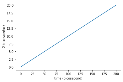
We can plot the trajectory of the system along the \(X\) axis:

plt.plot(traj_dict['time'], traj_dict['coordinates'][:,0,0])
plt.xlabel('time ({})'.format(traj_dict['time'].unit))
plt.ylabel('X ({})'.format(traj_dict['coordinates'].unit))
plt.show()

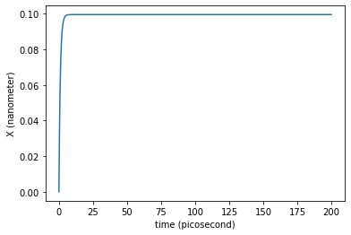
traj_dict = langevin(molecular_system,
                     friction=1.0/unit.picoseconds,
                     temperature=0.0*unit.kelvin,
                     time=0.2*unit.nanoseconds,
                     saving_timestep=0.10*unit.picoseconds,
                     integration_timestep=0.01*unit.picoseconds)

plt.plot(traj_dict['time'], traj_dict['coordinates'][:,0,0])
plt.xlabel('time ({})'.format(traj_dict['time'].unit))
plt.ylabel('X ({})'.format(traj_dict['coordinates'].unit))
plt.show()

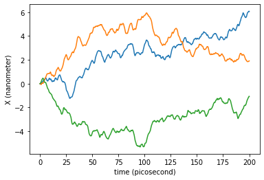
Langevin dynamics

traj_dict = langevin(molecular_system,
                     friction=1.0/unit.picoseconds,
                     temperature=300.0*unit.kelvin,
                     time=0.2*unit.nanoseconds,
                     saving_timestep=0.10*unit.picoseconds,
                     integration_timestep=0.01*unit.picoseconds)

We represent now the stochastic trajectory of our free particle along the axis \(X\) in time:

plt.plot(traj_dict['time'], traj_dict['coordinates'][:,0,0])
plt.plot(traj_dict['time'], traj_dict['coordinates'][:,0,1])
plt.plot(traj_dict['time'], traj_dict['coordinates'][:,0,2])
plt.xlabel('time ({})'.format(traj_dict['time'].unit))
plt.ylabel('X ({})'.format(traj_dict['coordinates'].unit))
plt.show()

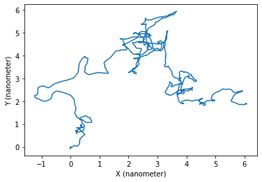
Or over the plane \(X,Y\):

plt.plot(traj_dict['coordinates'][:,0,0], traj_dict['coordinates'][:,0,1])
plt.xlabel('X ({})'.format(traj_dict['coordinates'].unit))
plt.ylabel('Y ({})'.format(traj_dict['coordinates'].unit))
plt.show()