Molecular dynamics

With OpenMM

import openmm as mm
from openmm import unit
from uibcdf_systems import HarmonicWell

molecular_system = HarmonicWell(n_particles = 1, mass = 32 * unit.amu,
                                k=5.0 * unit.kilocalories_per_mole/unit.nanometers**2)

integrator = mm.LangevinIntegrator(300.0*unit.kelvin, 1.0/unit.picoseconds, 0.02*unit.picoseconds)
platform = Platform.getPlatformByName('CUDA')
simulation = Simulation(molecular_system.topology, molecular_system.system, integrator, platform)

coordinates = np.zeros([1, 3], np.float32) * unit.nanometers
simulation.context.setPositions()

velocities = np.zeros([1, 3], np.float32) * unit.nanometers/unit.picoseconds
simulation.context.setVelocities()

simulation.step(1000)

With this library

Newtonian dynamics

import numpy as np
import sympy as sy
import matplotlib.pyplot as plt
from openmm import unit

---------------------------------------------------------------------------
ModuleNotFoundError                       Traceback (most recent call last)
/tmp/ipykernel_3840/3413763320.py in <module>
      1 import numpy as np
      2 import sympy as sy
----> 3 import matplotlib.pyplot as plt
      4 from openmm import unit

ModuleNotFoundError: No module named 'matplotlib'

from uibcdf_systems import HarmonicWell
from uibcdf_systems.tools import langevin

molecular_system = HarmonicWell(n_particles = 1, mass = 32 * unit.amu,
                                k=5.0 * unit.kilocalories_per_mole/unit.nanometers**2)

initial_positions = np.zeros([1, 3], np.float32) * unit.nanometers
initial_positions[0,0] = 1.0 * unit.nanometers

initial_velocities = np.zeros([1, 3], np.float32) * unit.nanometers/unit.picoseconds

molecular_system.set_coordinates(initial_positions)
molecular_system.set_velocities(initial_velocities)

traj_dict = langevin(molecular_system,
                     friction=0.0/unit.picoseconds,
                     temperature=0.0*unit.kelvin,
                     time=50.0*unit.picoseconds,
                     saving_timestep=0.1*unit.picoseconds,
                     integration_timestep=0.005*unit.picoseconds)

We can now plot the trajectory of the x coordinate:

plt.plot(traj_dict['time'], traj_dict['coordinates'][:,0,0])
plt.xlabel('time ({})'.format(traj_dict['time'].unit))
plt.ylabel('X ({})'.format(traj_dict['coordinates'].unit))
plt.show()

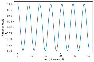
We can wonder now if the period of these oscillations is in agreement with the value calculated above.

mass = molecular_system.parameters['mass']
k = molecular_system.parameters['k']
T = 2*np.pi*np.sqrt(mass/k)

print('The period of the small oscillations around the minimum is',T)

The period of the small oscillations around the minimum is 7.770948260727904 ps

molecular_system.get_oscillations_time_period()

Quantity(value=7.770948260727904, unit=picosecond)

plt.plot(traj_dict['time'], traj_dict['coordinates'][:,0,0])
plt.axvline(T._value, color='gray', linestyle='--') # Period of the harmonic oscillations
plt.xlabel('time ({})'.format(traj_dict['time'].unit))
plt.ylabel('X ({})'.format(traj_dict['coordinates'].unit))
plt.show()

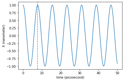
Remember that the integration timestep must be smaller than \(\sim T/10.0\) to guarantee that no artifacts are introduced by the timestep size.

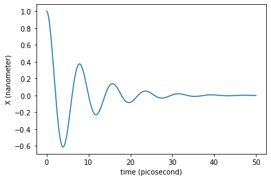
The newtonian dynamics can also include damping. This way we can simulate damped oscillations around the minimum.

traj_dict = langevin(molecular_system,
                     friction=0.25/unit.picoseconds,
                     temperature=0.0*unit.kelvin,
                     time=50.0*unit.picoseconds,
                     saving_timestep=0.1*unit.picoseconds,
                     integration_timestep=0.02*unit.picoseconds)

plt.plot(traj_dict['time'], traj_dict['coordinates'][:,0,0])
plt.xlabel('time ({})'.format(traj_dict['time'].unit))
plt.ylabel('X ({})'.format(traj_dict['coordinates'].unit))
plt.show()

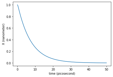
What would be the friction value needed to enter in the overdamped regime?

traj_dict = langevin(molecular_system,
                     friction=5.0/unit.picoseconds,
                     temperature=0.0*unit.kelvin,
                     time=50.0*unit.picoseconds,
                     saving_timestep=0.1*unit.picoseconds,
                     integration_timestep=0.02*unit.picoseconds)

plt.plot(traj_dict['time'], traj_dict['coordinates'][:,0,0])
plt.xlabel('time ({})'.format(traj_dict['time'].unit))
plt.ylabel('X ({})'.format(traj_dict['coordinates'].unit))
plt.show()

Langevin dynamics

traj_dict = langevin(molecular_system,
                     friction=1.0/unit.picoseconds,
                     temperature=300.0*unit.kelvin,
                     time=1.0*unit.nanoseconds,
                     saving_timestep=0.5*unit.picoseconds,
                     integration_timestep=0.02*unit.picoseconds)

Let us see the time evolution of the coordinate \(x\) of our single particle:

plt.plot(traj_dict['time'], traj_dict['coordinates'][:,0,0])
plt.xlabel('time ({})'.format(traj_dict['time'].unit))
plt.ylabel('X ({})'.format(traj_dict['coordinates'].unit))
plt.show()

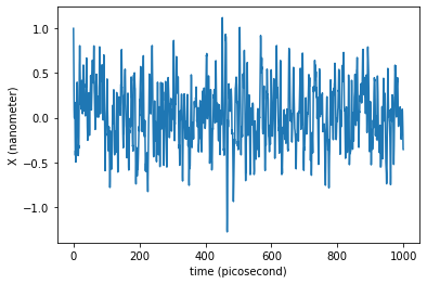
molecular_system.get_standard_deviation(300.0*unit.kelvin)

Quantity(value=0.34530023967331663, unit=nanometer)

np.std(traj_dict['coordinates'][:,0,0])

Quantity(value=0.34393127752734576, unit=nanometer)