import numpy as np
import sympy as sy
import matplotlib.pyplot as plt
from openmm import unit
---------------------------------------------------------------------------
ModuleNotFoundError                       Traceback (most recent call last)
/tmp/ipykernel_3819/3413763320.py in <module>
      1 import numpy as np
      2 import sympy as sy
----> 3 import matplotlib.pyplot as plt
      4 from openmm import unit

ModuleNotFoundError: No module named 'matplotlib'
Harmonic well potential
The harmonic well potential is described by the following expression:
Where \(k\) is the only parameter and represents the stiffness of the harmonic potential -or the stiffness of the harmonic spring described by the hookes’ law-. Notice that the potential for potential dimensions \(Y\) and \(Z\), has the same shape. In this way we have a three dimensional harmonic well. But let’s see here only the proyection over a single dimension \(X\) since \(Y\) and \(Z\) are decorrelated, and there by will behave as \(X\).
def harmonic_well(x,k):
    return 0.5*k*x**2
k=5.0 * unit.kilocalories_per_mole/ unit.nanometers**2 # stiffness of the harmonic potential

x_serie = np.arange(-5., 5., 0.05) * unit.nanometers

plt.plot(x_serie, harmonic_well(x_serie, k), 'r-')
plt.ylim(-1,5)
plt.xlim(-2,2)
plt.grid()
plt.xlabel("X ({})".format(unit.nanometers))
plt.ylabel("Energy ({})".format(unit.kilocalories_per_mole))
plt.title("Harmonic Well")
plt.show()
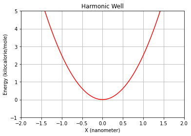
Different values of \(k\) can be tested to graphically see how this parameter accounts for the openness of the well’s arms. Or, as it is described below, the period of oscillations of a particle of mass \(m\) in a newtonian dynamics.
The hooks’ law describes the force suffered by a mass attached to an ideal spring as:
Where \(k\) is the stiffness of the spring and \(x_{0}\) is the equilibrium position. Now, since the force is minus the gradient of the potential energy \(V(x)\),
we can proof that the spring force is the result of the first harmonic potential derivative:
And the angular frequency of oscillations of a spring, or a particle goberned by the former potential, is:
Where \(m\) is the mass of the particle. This way the potential can also be written as:
Finnally, the time period of these oscillations are immediately computed from the mass of the particle, \(m\), and the stiffness parameter \(k\). Given that by definition:
Then:
