Principal Component Analysis#

Computing covariance eigenvectors and eigenvalues to identify principal conformational motions.

The function molsysmt.structure.principal_component_analysis() performs essential dynamics (PCA) by constructing and diagonalizing the Cartesian atomic positional covariance matrix across a trajectory, extracting the principal collective modes of conformational motion.

Added in version 1.0.0.

API documentation

Follow this link for a detailed description of the input arguments, raised errors, and returned objects of this function: molsysmt.structure.principal_component_analysis().

Basic usage#

Let’s show how to perform principal component analysis on a pentalanine trajectory (fitting frames first to isolate internal conformational dynamics from rotational/translational drift):

import molsysmt as msm
import matplotlib.pyplot as plt
import pyunitwizard as puw
import numpy as np

molsys = msm.convert(msm.systems['pentalanine']['traj_pentalanine.h5msm'])
molsys_fitted = msm.structure.least_rmsd_fit(molsys, selection='all', selection_fit='backbone', reference_structure_index=0)

Note

Demo Systems Catalog

This tutorial uses demonstration datasets provided by MolSysMT. To explore the full catalog of bundled systems, forms, and file paths, visit the Demo Systems guide.

We compute the covariance eigenvectors and eigenvalues for heavy atoms using molsysmt.structure.principal_component_analysis():

eigenvectors, eigenvalues = msm.structure.principal_component_analysis(molsys_fitted, selection='atom_type!="H"')

print('Eigenvectors shape (modes x 3*atoms):', eigenvectors.shape)
print('Eigenvalues shape (variances):', eigenvalues.shape)
print('Top 3 eigenvalues:', eigenvalues[:3])

Eigenvectors shape (modes x 3*atoms): (90, 90)
Eigenvalues shape (variances): (90,)
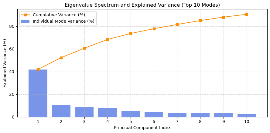
Top 3 eigenvalues: [0.5964943862487921 0.14677595412969768 0.1194879104451236] nanometer ** 2

Cumulative explained variance and eigenvalue spectrum#

We compute and plot the individual and cumulative explained variance ratios to assess how many principal components capture the majority of the conformational motion:

eig_vals = puw.get_value(eigenvalues)
var_ratio = eig_vals / np.sum(eig_vals)
cum_var = np.cumsum(var_ratio)

plt.figure(figsize=(9, 4.5))
plt.plot(range(1, 11), cum_var[:10] * 100, marker='s', color='darkorange', lw=1.5, label='Cumulative Variance (%)')
plt.bar(range(1, 11), var_ratio[:10] * 100, color='royalblue', alpha=0.7, label='Individual Mode Variance (%)')
plt.xlabel('Principal Component Index')
plt.ylabel('Explained Variance (%)')
plt.title('Eigenvalue Spectrum and Explained Variance (Top 10 Modes)')
plt.xticks(range(1, 11))
plt.grid(True, linestyle='--', alpha=0.5)
plt.legend()
plt.tight_layout()
plt.show()

../../../../_images/4d8b8c57f23addbb8293b8c8efd4a587a70964d9e58616503466b65639c20944.png

Projecting structural ensembles onto principal components#

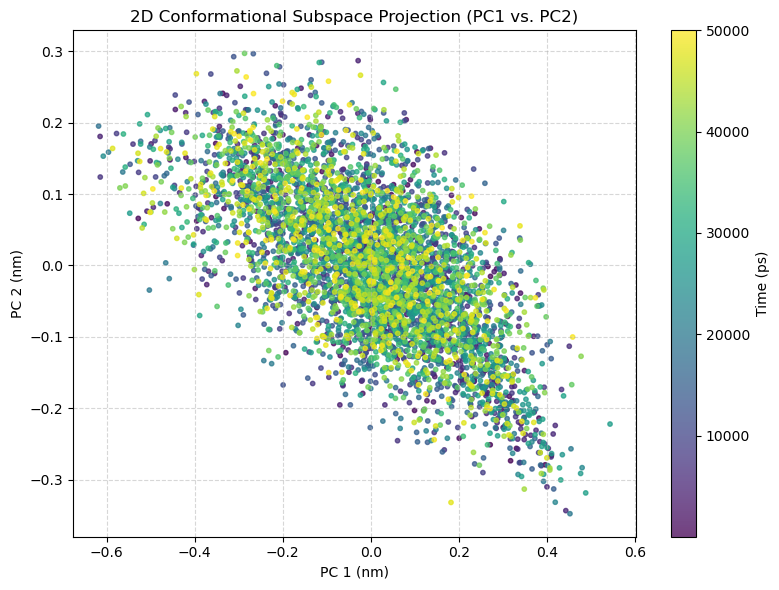
We project the trajectory structures onto the top two principal components (PC1 and PC2) to map the low-dimensional conformational energy landscape:

coords = msm.get(molsys_fitted, element='atom', selection='atom_type!="H"', coordinates=True)
coords_val = puw.get_value(coords, to_unit='nm')
n_structures, n_atoms, _ = coords_val.shape
flat_coords = coords_val.reshape(n_structures, n_atoms * 3)
mean_coords = np.mean(flat_coords, axis=0)
centered = flat_coords - mean_coords

pc1_proj = np.dot(centered, eigenvectors[0])
pc2_proj = np.dot(centered, eigenvectors[1])
time = puw.get_value(msm.get(molsys, element='system', time=True), to_unit='ps')

plt.figure(figsize=(8, 6))
scatter = plt.scatter(pc1_proj, pc2_proj, c=time, cmap='viridis', s=10, alpha=0.75)
cbar = plt.colorbar(scatter)
cbar.set_label('Time (ps)')
plt.xlabel('PC 1 (nm)')
plt.ylabel('PC 2 (nm)')
plt.title('2D Conformational Subspace Projection (PC1 vs. PC2)')
plt.grid(True, linestyle='--', alpha=0.5)
plt.tight_layout()
plt.show()

../../../../_images/9525b3ca498d28bb7e0bbdd5041669263bbc9d517da74d117fe576454505df0b.png