Working with OpenMM#

Setting up, parametrizing, simulating, and streaming molecular dynamics trajectories from MolSysMT to OpenMM.

MolSysMT seamlessly integrates with OpenMM, allowing computational biophysicists to move effortlessly from raw experimental coordinates to energy minimization, equilibration, and production MD simulations.

In this recipe, we prepare the Villin Headpiece miniprotein, add missing caps and hydrogens, solvate it, construct an OpenMM Simulation context using direct MolSysMT conversion gateways, attach native reporters, execute a simulation run, and analyze the trajectory.

Added in version 1.0.0.

System Preparation#

We start by loading the Villin Headpiece structure, capping terminals, adding hydrogens, and solvating in a cubic box with 0.10 M NaCl:

import molsysmt as msm

# Load Villin Headpiece from bundled systems
molsys = msm.convert(msm.systems['chicken villin HP35']['chicken_villin_HP35.h5msm'], to_form='molsysmt.MolSys')
molsys = msm.build.add_missing_terminal_cappings(molsys)
molsys = msm.build.add_missing_hydrogens(molsys)

# Solvate with AMBER14 and TIP3P in a cubic box with 1.0 nm clearance
solvated_molsys = msm.build.solvate(
    [molsys, {'forcefield': 'AMBER14', 'water_model': 'TIP3P'}],
    box_shape='cubic',
    clearance='10.0 angstroms',
    to_form='molsysmt.MolSys',
    engine='OpenMM'
)

msm.info(solvated_molsys)

form	n_atoms	n_groups	n_components	n_chains	n_molecules	n_entities	n_waters	n_ions	n_peptides	n_structures
molsysmt.MolSys	7231	2248	2211	2	2211	3	2208	2	1	1

Viewing Solvated System#

We visualize the solvated protein before starting the simulation:

msm.view(solvated_molsys)

Creating OpenMM Objects#

We convert our prepared system directly into OpenMM native objects (openmm.Topology and openmm.System) via MolSysMT converters:

from openmm import app, unit, LangevinIntegrator, Platform
from molsysmt import pyunitwizard as puw

# Direct conversion to openmm.Topology and openmm.System
openmm_topology = msm.convert(solvated_molsys, to_form='openmm.Topology')
system = msm.convert(
    solvated_molsys,
    to_form='openmm.System',
    forcefield='AMBER14',
    water_model='TIP3P',
    non_bonded_method='PME',
    constraints='hbonds'
)

# Extract and convert coordinate units
coordinates = msm.get(solvated_molsys, coordinates=True)
positions = puw.convert(coordinates[0], to_form='openmm.unit')

print(f"OpenMM System created with {system.getNumParticles()} particles.")

OpenMM System created with 7231 particles.

Configuring Simulation#

We configure Langevin dynamics at 300 K, attach native MolSysMT reporters, and minimize potential energy:

# Integrator: Langevin dynamics at 300 K
integrator = LangevinIntegrator(300*unit.kelvin, 1.0/unit.picosecond, 2.0*unit.femtoseconds)
platform = Platform.getPlatformByName('CPU')
simulation = app.Simulation(openmm_topology, system, integrator, platform)
simulation.context.setPositions(positions)

# Energy minimization
simulation.minimizeEnergy(maxIterations=20)

# Attach MolSysMT StructuresDict reporter with periodic box tracking
from molsysmt.third_party.openmm.reporters import StructuresDictReporter

structures_reporter = StructuresDictReporter(10, box=True)
simulation.reporters.append(structures_reporter)

Running Simulation#

We execute the simulation steps and extract the collected frames into memory:

# Execute MD steps
simulation.step(50)

# Finalize reporter and construct MolSys trajectory
traj_dict = structures_reporter.finalize()
traj_molsys = msm.convert([solvated_molsys.topology, traj_dict], to_form='molsysmt.MolSys')

print(f"Captured {msm.get(traj_molsys, n_structures=True)} frames in memory.")

Captured 6 frames in memory.

Trajectory Analysis#

We calculate the C-alpha backbone RMSD progression across the simulation frames:

# Compute RMSD over the generated trajectory
rmsd_values = msm.structure.get_rmsd(
    traj_molsys,
    selection='atom_name=="CA"',
    reference_structure_index=0
)
rmsd_nm = [msm.pyunitwizard.get_value(val, to_unit='nm') for val in rmsd_values]
print("Backbone RMSD progression (nm):", [f"{v:.4f}" for v in rmsd_nm])

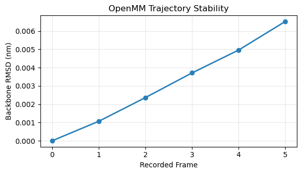
Backbone RMSD progression (nm): ['0.0000', '0.0011', '0.0024', '0.0037', '0.0050', '0.0065']

Plotting RMSD Profile#

We plot the RMSD progression over the collected frames:

import matplotlib.pyplot as plt

fig, ax = plt.subplots(figsize=(6, 3.5))
frame_indices = range(len(rmsd_nm))
ax.plot(frame_indices, rmsd_nm, marker='o', color='#2980B9', linewidth=2)
ax.set_xlabel('Recorded Frame')
ax.set_ylabel('Backbone RMSD (nm)')
ax.set_title('OpenMM Trajectory Stability')
ax.grid(True, alpha=0.3)
plt.tight_layout()
plt.show()